---
title: "Design for fitting MMRM"
author: "Daniel Sabanes Bove"
output: html_document
editor_options:
  chunk_output_type: console
---

```{r setup, include=FALSE}
knitr::opts_chunk$set(echo = TRUE)
```

# Objective

We would like to prototype the whole flow of fitting an MMRM in this new package.
This will make subsequent issue solutions more efficient.

```{r}
library(mmrm)
library(checkmate)
library(glmmTMB)
```

# Example

Let's first set up some example.

```{r}
dat <- fev_data
vs <- list(
  response = "FEV1",
  covariates = c("RACE", "SEX"),
  id = "USUBJID",
  arm = "ARMCD",
  visit = "AVISIT"
)
```

# Prototypes

## `check_vars()` --> `h_labels()` and `assert_data()`

We try to simplify the function compared to the old code, using external helpers
and splitting up the function.

```{r}
h_is_specified <- function(x, vars) {
  !is.null(vars[[x]])
}
h_is_specified_and_in_data <- function(x, vars, data) {
  h_is_specified(x, vars) && all(vars[[x]] %in% names(data))
}
h_check_and_get_label <- function(x, vars, data) {
  assert_true(h_is_specified_and_in_data(x, vars, data))
  res <- NULL
  for (v in vars[[x]]) {
    label <- attr(data[[v]], "label")
    string <- ifelse(!is.null(label), label, v)
    res <- c(res, stats::setNames(string, v))
  }
  res
}
h_get_covariate_parts <- function(covariates) {
  unique(unlist(strsplit(covariates, split = "\\*|:")))
}
```

Let's quickly try these out:

```{r}
h_check_and_get_label("arm", vs, dat)
```

Let's have a separate `h_labels()` function. This is mostly checking
the variable specifications on the side, too.

```{r}
h_labels <- function(vars,
                     data) {
  assert_list(vars)
  assert_data_frame(data)

  labels <- list()

  labels$response <- h_check_and_get_label("response", vars, data)
  labels$id <- h_check_and_get_label("id", vars, data)
  labels$visit <- h_check_and_get_label("visit", vars, data)
  if (h_is_specified("arm", vars)) {
    h_check_and_get_label("arm", vars, data)
  }
  if (h_is_specified("covariates", vars)) {
    vars$parts <- h_get_covariate_parts(vars$covariates)
    labels$parts <- h_check_and_get_label("parts", vars, data)
  }

  return(labels)
}

h_labels(vs, dat)
```

Now let's do the check (assertion) function for the data.
Again let's brake it down into manageable pieces.

```{r}
h_assert_one_rec_pt_visit <- function(vars, data) {
  # Check there is no more than one record per patient and visit.
  form <- stats::as.formula(paste("~", vars$visit, "+", vars$id))
  grouped_data <- split(data, f = form)
  n_per_group <- vapply(grouped_data, nrow, integer(1))

  if (any(n_per_group > 1)) {
    dupl_group <- which(n_per_group > 1)
    n_dupl <- length(dupl_group)
    stop(paste(
      "There are", n_dupl, "subjects with more than one record per visit:",
      toString(names(n_dupl))
    ))
  }
}

h_assert_rsp_var <- function(vars, data) {
  response_values <- data[[vars$response]]
  assert_numeric(response_values)
}

h_assert_visit_var <- function(vars, data) {
  visit_values <- data[[vars$visit]]
  assert_factor(visit_values)
}

assert_data <- function(vars, data) {
  assert_list(vars)
  assert_data_frame(data)

  # First subset data to observations with complete regressors.
  regressor_vars <- c(vars$arm, vars$visit, h_get_covariate_parts(vars$covariates))
  has_complete_regressors <- stats::complete.cases(data[, regressor_vars])
  data_complete_regressors <- droplevels(data[has_complete_regressors, ])

  h_assert_one_rec_pt_visit(vars, data_complete_regressors)
  h_assert_rsp_var(vars, data_complete_regressors)
  h_assert_visit_var(vars, data_complete_regressors)

  # Second only look at complete data.
  has_complete_response <- stats::complete.cases(data_complete_regressors[, vars$response])
  data_complete <- droplevels(data_complete_regressors[has_complete_response, ])

  if (h_is_specified("arm", vars)) {
    assert_factor(data_complete_regressors[[vars$arm]], min.levels = 2L)
    assert_factor(
      data_complete[[vars$arm]],
      levels = levels(data_complete_regressors[[vars$arm]])
    )
    assert_true(all(table(data_complete[[vars$arm]]) > 5))
  } else {
    assert_data_frame(data_complete, min.rows = 5L)
  }
}
```

Note that in production the arm checking part could be also put into a
helper function to make the `assert_data()` function more consistent.

Now let's try this out, too.

```{r}
assert_data(vs, dat)
```


## `h_build_formula()`

Let's build the formula for the `glmmTMB` fit call. Basically we want something
like this:

`AVAL ~ STRATA1 + BMRKR2 + ARMCD + ARMCD + AVISIT + ARMCD * AVISIT + us(0 + AVISIT | USUBJID)`

where the `us` part would look different for covariance structures other than
this unstructured one.

For the `cor_struct` argument we keep a bit more higher level syntax than
`glmmTMB` itself, since e.g. `us` and `cs` could easily be confused by the user.

Note that for now we don't put in the option to have separate covariance matrices
per group yet, we can do this in a second pass later on (backlog).

```{r}
h_build_formula <- function(vars,
                            cor_struct = c(
                              "unstructured",
                              "toeplitz",
                              "auto-regressive",
                              "compound-symmetry"
                            )) {
  assert_list(vars)
  cor_struct <- match.arg(cor_struct)

  covariates_part <- paste(
    vars$covariates,
    collapse = " + "
  )
  arm_visit_part <- if (is.null(vars$arm)) {
    vars$visit
  } else {
    paste0(
      vars$arm,
      "*",
      vars$visit
    )
  }
  random_effects_fun <- switch(cor_struct,
    "unstructured" = "us",
    "toeplitz" = "toep",
    "auto-regressive" = "ar1",
    "compound-symmetry" = "cs"
  )
  random_effects_part <- paste0(
    random_effects_fun, "(0 + ", vars$visit, " | ", vars$id, ")"
  )
  rhs_formula <- paste(
    arm_visit_part,
    "+",
    random_effects_part
  )
  if (covariates_part != "") {
    rhs_formula <- paste(
      covariates_part,
      "+",
      rhs_formula
    )
  }
  stats::as.formula(paste(
    vars$response,
    "~",
    rhs_formula
  ))
}
```

Let's try this out:

```{r}
h_build_formula(vs, "toeplitz")
h_build_formula(vs)
```

## `h_cov_estimate()`

Let's see if we even need this function.

```{r}
mod <- glmmTMB(
  FEV1 ~ ar1(0 + AVISIT | USUBJID),
  data = dat,
  dispformula = ~0,
  REML = TRUE
)
vc <- VarCorr(mod)
vc$cond[[1]]
class(mod) <- c("mmrm_fit", "glmmTMB")
```

OK so that is still not super intuitive, so let's better have the function.
Especially as we also want to return how many variance parameters
there are. For backwards compatibility we also return one ID which had the
maximum number of visits. Maybe later we can remove this again.

```{r}
h_cov_estimate <- function(model) {
  assert_class(model, "mmrm_fit")

  cov_est <- VarCorr(model)$cond[[1L]]
  theta <- getME(model, "theta")
  id_per_obs <- model$modelInfo$reTrms$cond$flist[[1L]]
  n_visits <- length(model$modelInfo$reTrms$cond$cnms[[1L]])
  which_id <- which(table(id_per_obs) == n_visits)[1L]

  structure(
    cov_est,
    id = levels(id_per_obs)[which_id],
    n_parameters = length(theta)
  )
}

str(h_cov_estimate(mod))
```

Here we also get the standard deviations and the correlation matrix as
attributes but that seems useful.

## `h_record_all_output()`

This is direct copy, and then slightly modified, from `rbmi`.
Therefore we need to include its author (Craig) as contributors in `mmrm`.

```{r}
#' Capture all Output
#'
#' This function silences all warnings, errors & messages and instead returns a list
#' containing the results (if it didn't error) + the warning and error messages as
#' character vectors.
#'
#' @param expr (`expression`)\cr to be executed.
#' @param remove (`list`)\cr optional list with elements `warnings`, `errors`,
#'   `messages` which can be character vectors, which will be removed from the
#'   results if specified.
#'
#' @return
#' A list containing
#'
#' - `result`: The object returned by `expr` or `list()` if an error was thrown
#' - `warnings`: `NULL` or a character vector if warnings were thrown.
#' - `errors`: `NULL` or a string if an error was thrown.
#' - `messages`: `NULL` or a character vector if messages were produced.
#'
#' @examples
#' \dontrun{
#' h_record_all_output({
#'   x <- 1
#'   y <- 2
#'   warning("something went wrong")
#'   message("O nearly done")
#'   x + y
#' })
#' }
h_record_all_output <- function(expr, remove = list()) {
  # Note: We don't need to and cannot assert `expr` here.
  assert_list(remove)

  env <- new.env()
  result <- withCallingHandlers(
    withRestarts(
      expr,
      muffleStop = function() list()
    ),
    message = function(m) {
      msg_without_newline <- gsub(m$message, pattern = "\n$", replacement = "")
      env$message <- c(env$message, msg_without_newline)
      invokeRestart("muffleMessage")
    },
    warning = function(w) {
      env$warning <- c(env$warning, w$message)
      invokeRestart("muffleWarning")
    },
    error = function(e) {
      env$error <- c(env$error, e$message)
      invokeRestart("muffleStop")
    }
  )
  list(
    result = result,
    warnings = setdiff(env$warning, remove$warnings),
    errors = setdiff(env$error, remove$errors),
    messages = setdiff(env$message, remove$messages)
  )
}

h_record_all_output(
  {
    x <- 1
    y <- 2
    warning("something went wrong")
    message("O nearly done")
    message("Almost done")
    x + y
  },
  remove = list(messages = c("Almost done", "bla"))
)
```


## `fit_single_optimizer()`

Here the optimizers are possible multivariate ones for `stats::optim()`, with
the default changed to `L-BFGS-B`. Note that we removed the `SANN` option since
that needs very long computation times, so does not seem practical.

We provide the new possibility for starting values.

While this function is not the primary user interface, it can be helpful for users.
Therefore we don't prefix with `h_`.

```{r}
fit_single_optimizer <- function(formula,
                                 data,
                                 start = NULL,
                                 optimizer = c("L-BFGS-B", "Nelder-Mead", "BFGS", "CG")) {
  assert_formula(formula)
  assert_data_frame(data)
  assert_list(start, null.ok = TRUE)
  optimizer <- match.arg(optimizer)

  control <- glmmTMB::glmmTMBControl(
    optimizer = stats::optim,
    optArgs = list(method = optimizer),
    parallel = 1L
  )
  quiet_fit <- h_record_all_output(
    glmmTMB::glmmTMB(
      formula = formula,
      data = data,
      dispformula = ~0,
      REML = TRUE,
      start = start,
      control = control
    ),
    remove = list(
      warnings = c(
        "OpenMP not supported.",
        "'giveCsparse' has been deprecated; setting 'repr = \"T\"' for you"
      )
    )
  )
  converged <- (length(quiet_fit$warnings) == 0L) &&
    (length(quiet_fit$errors) == 0L) &&
    (quiet_fit$result$fit$convergence == 0)
  structure(
    quiet_fit$result,
    errors = quiet_fit$errors,
    warnings = quiet_fit$warnings,
    messages = quiet_fit$messages,
    optimizer = optimizer,
    converged = converged,
    class = c("mmrm_fit", class(quiet_fit$result))
  )
}
```

OK let's try this one out:

```{r}
mod_fit <- fit_single_optimizer(
  formula = h_build_formula(vs),
  data = dat
)
attr(mod_fit, "converged")
```

Looks good so far!

## `h_summarize_all_fits()`

Note that we don't return the fixed effects as that is not used downstream.

```{r}
h_summarize_all_fits <- function(all_fits) {
  assert_list(all_fits)

  warnings <- lapply(all_fits, attr, which = "warnings")
  messages <- lapply(all_fits, attr, which = "messages")
  log_liks <- vapply(all_fits, stats::logLik, numeric(1L))
  converged <- vapply(all_fits, attr, logical(1), which = "converged")

  list(
    warnings = warnings,
    messages = messages,
    log_liks = log_liks,
    converged = converged
  )
}

h_summarize_all_fits(list(mod_fit, mod_fit))
```

## `h_free_cores()`

This is from the `tern.mmrm` package. Since Daniel wrote this function and
we will take it out of `tern.mmrm` before publishing no further author
implications.

Note that we will need to add the `parallel` and `utils` packages to `Imports`.

```{r}
#' Get an approximate number of free cores.
#'
#' @return the approximate number of free cores, which is an integer between 1 and one less than
#'   the total cores.
#'
#' @details This uses the maximum load average at 1, 5 and 15 minutes on Linux and Mac
#'   machines to approximate the number of busy cores. For Windows, the load percentage is
#'   multiplied with the total number of cores.
#'   We then subtract this from the number of all detected cores. One additional core
#'   is not used for extra safety.
#'
#' @noRd
h_free_cores <- function() {
  all_cores <- parallel::detectCores(all.tests = TRUE)
  busy_cores <-
    if (.Platform$OS.type == "windows") {
      load_percent_string <- system("wmic cpu get loadpercentage", intern = TRUE)
      # This gives e.g.: c("LoadPercentage", "10", "")
      # So we just take the number here.
      load_percent <- as.integer(min(load_percent_string[2L], 100))
      assert_int(load_percent, lower = 0, upper = 100)
      ceiling(all_cores * load_percent / 100)
    } else if (.Platform$OS.type == "unix") {
      uptime_string <- system("uptime", intern = TRUE)
      # This gives e.g.:
      # "11:00  up  1:57, 3 users, load averages: 2.71 2.64 2.62"
      # Here we just want the last three numbers.
      uptime_split <- strsplit(uptime_string, split = ",|\\s")[[1]] # Split at comma or white space.
      uptime_split <- uptime_split[uptime_split != ""]
      load_averages <- as.numeric(utils::tail(uptime_split, 3))
      ceiling(max(load_averages))
    }
  assert_number(all_cores, lower = 1, finite = TRUE)
  assert_number(busy_cores, lower = 0, upper = all_cores)

  # For safety, we subtract 1 more core from all cores.
  as.integer(max(1, all_cores - busy_cores - 1))
}

h_free_cores()
```

Right now e.g. I have total 16 cores, and I get 14 returned by this function
which makes sense (1 is busy, and 1 is extra buffer).

## `refit_multiple_optimizers()`

```{r}
refit_multiple_optimizers <- function(fit,
                                      n_cores = 1L,
                                      optimizers = c("L-BFGS-B", "Nelder-Mead", "BFGS", "CG")) {
  assert_class(fit, "mmrm_fit")
  assert_int(n_cores, lower = 1L)
  optimizers <- match.arg(optimizers, several.ok = TRUE)

  # Extract the components of the original fit.
  old_formula <- stats::formula(fit)
  old_data <- fit$frame
  old_optimizer <- attr(fit, "optimizer")

  # Settings for the new fits.
  optimizers <- setdiff(optimizers, old_optimizer)
  n_cores_used <- ifelse(
    .Platform$OS.type == "windows",
    1L,
    min(
      length(optimizers),
      n_cores
    )
  )

  all_fits <- parallel::mclapply(
    X = optimizers,
    FUN = fit_single_optimizer,
    formula = old_formula,
    data = old_data,
    start = list(theta = fit$fit$par), # Take the results from old fit as starting values.
    mc.cores = n_cores_used,
    mc.silent = TRUE
  )
  names(all_fits) <- optimizers
  all_fits_summary <- h_summarize_all_fits(all_fits)

  # Find the results that are ok:
  is_ok <- all_fits_summary$converged
  if (!any(is_ok)) {
    stop(
      "No optimizer led to a successful model fit. ",
      "Please try to use a different covariance structure or other covariates."
    )
  }

  # Return the best result in terms of log-likelihood.
  best_optimizer <- names(which.max(all_fits_summary$log_liks[is_ok]))
  best_fit <- all_fits[[best_optimizer]]
  return(best_fit)
}
```

OK, let's try this out. Say we don't converge with the first optimizer choice,
and then want to run multiple ones.

```{r}
mod_fit <- fit_single_optimizer(
  formula = h_build_formula(vs),
  data = dat,
  optimizer = "Nelder-Mead"
)
attr(mod_fit, "converged")
attr(mod_fit, "warnings")
```

So Nelder-Mead does not converge, and we see a non-positive-definite Hessian
warning.
Now we put this into the refit function:

```{r}
mod_refit <- refit_multiple_optimizers(mod_fit)
```

## `fit_model()`

This is wrapping the lower level fitting functions (single and multiple optimizers).

```{r}
fit_model <- function(formula,
                      data,
                      optimizer = "automatic",
                      n_cores = 1L) {
  assert_string(optimizer)
  use_automatic <- identical(optimizer, "automatic")

  fit <- fit_single_optimizer(
    formula = formula,
    data = data,
    optimizer = ifelse(use_automatic, "L-BFGS-B", optimizer)
  )

  if (attr(fit, "converged")) {
    fit
  } else if (use_automatic) {
    refit_multiple_optimizers(fit, n_cores = n_cores)
  } else {
    all_problems <- unlist(
      attributes(fit)[c("errors", "messages", "warnings")],
      use.names = FALSE
    )
    stop(paste0(
      "Chosen optimizer '", optimizer, "' led to problems during model fit:\n",
      paste(paste0(seq_along(all_problems), ") ", all_problems), collapse = ";\n"), "\n",
      "Consider using the 'automatic' optimizer."
    ))
  }
}
```

Let's try this out quickly too:

```{r}
testthat::expect_error(fit_model(
  formula = h_build_formula(vs),
  data = dat,
  optimizer = "Nelder-Mead"
))
```

So this gives the expected error message.

```{r}
mod_fit2 <- fit_model(
  formula = h_build_formula(vs),
  data = dat,
  optimizer = "BFGS"
)
```

And this works.

## `vars()`

Just a little user interface list generator for the variables to use in `mmrm()`.

```{r}
vars <- function(response = "AVAL",
                 covariates = c(),
                 id = "USUBJID",
                 arm = "ARM",
                 visit = "AVISIT") {
  list(
    response = response,
    covariates = covariates,
    id = id,
    arm = arm,
    visit = visit
  )
}

vars()
```

## `h_vcov_theta()`

This helper function returns the covariance estimate for the variance parameters
(`theta`) of the fitted MMRM.

```{r}
h_vcov_theta <- function(model) {
  assert_class(model, "mmrm_fit")

  model_vcov <- vcov(model, full = TRUE)
  theta <- getME(model, "theta")
  index_theta <- seq(to = nrow(model_vcov), length = length(theta))

  unname(model_vcov[index_theta, index_theta, drop = FALSE])
}

vcov_theta <- h_vcov_theta(mod_refit)
```

However one question is now which `theta` parametrization is used here
to provide the covariance matrix of. Because it is strange that these two
are not the same:

```{r}
mod_refit$obj$par
mod_refit$fit$par
```

It could be that the first one are the starting values for the optimization.
Indeed:

```{r}
identical(mod_fit$fit$par, mod_refit$obj$par)
```

## `h_num_vcov_theta()`

Let's see anyway if we can recover this covariance matrix also numerically:

```{r}
h_num_vcov_theta <- function(model) {
  assert_class(model, "mmrm_fit")

  theta_est <- model$fit$par
  devfun_theta <- model$obj$fn
  hess_theta <- numDeriv::hessian(func = devfun_theta, x = theta_est)
  eig_hess_theta <- eigen(hess_theta, symmetric = TRUE)
  with(eig_hess_theta, vectors %*% diag(1 / values) %*% t(vectors))
}

num_vcov_theta <- h_num_vcov_theta(mod_refit)
all.equal(vcov_theta, num_vcov_theta)
range(vcov_theta / num_vcov_theta)
```

So the results are quite different.

## `h_covbeta_fun()`

For below we need to construct a function `covbeta_fun` calculating
the covariance matrix for the fixed effects (`beta`) as a function of the
variance parameters.

```{r}
h_covbeta_fun <- function(model) {
  assert_class(model, "mmrm_fit")

  function(theta) {
    sdr <- TMB::sdreport(
      model$obj,
      par.fixed = theta,
      getJointPrecision = TRUE
    )
    q_mat <- sdr$jointPrecision
    which_fixed <- which(rownames(q_mat) == "beta")
    q_marginal <- glmmTMB:::GMRFmarginal(q_mat, which_fixed)
    unname(solve(as.matrix(q_marginal)))
  }
}
```

Let's try this out: We can recover the usual variance-covariance matrix of the
fixed effects when plugging in the estimated variance parameters (up to
reasonable numeric precision), and we get a different result when using
other variance parameters.

```{r}
covbeta_fun <- h_covbeta_fun(mod_refit)
mod_theta_est <- getME(mod_refit, "theta")
covbeta_num <- covbeta_fun(theta = mod_theta_est)
covbeta_fit <- unname(vcov(mod_refit)$cond)
all.equal(covbeta_num, covbeta_fit)
range(covbeta_num / covbeta_fit)
range(covbeta_num - covbeta_fun(theta = mod_theta_est * 0.9))
```

## `h_general_jac_list()`

We also need to compute the jacobian, and organize it as a list.

We start with a general helper that takes a function `covbeta_fun` (see above),
as well as `x_opt` which is the variance parameter estimate.

```{r}
h_general_jac_list <- function(covbeta_fun,
                               x_opt,
                               ...) {
  assert_function(covbeta_fun, nargs = 1L)
  assert_numeric(x_opt, any.missing = FALSE, min.len = 1L)

  jac_matrix <- numDeriv::jacobian(
    func = covbeta_fun,
    x = x_opt,
    # Note: No need to specify further `methods.args` here.
    ...
  )
  get_column_i_as_matrix <- function(i) {
    # This column contains the p x p entries.
    jac_col <- jac_matrix[, i]
    p <- sqrt(length(jac_col))
    # Obtain p x p matrix.
    matrix(jac_col, nrow = p, ncol = p)
  }
  lapply(
    seq_len(ncol(jac_matrix)),
    FUN = get_column_i_as_matrix
  )
}
```

Let's try this out, too:

```{r}
jac_example <- h_general_jac_list(covbeta_fun, mod_theta_est)
```

So this takes a few seconds to generate. However this is still in the same
ballpark as the fitting of the MMRM itself, so should not be practical problem.

## `h_jac_list()`

Now we can wrap this in a function that takes the fitted MMRM directly and
returns the Jacobian.

```{r}
h_jac_list <- function(model) {
  covbeta_fun <- h_covbeta_fun(model)
  theta_est <- getME(model, "theta")
  h_general_jac_list(covbeta_fun = covbeta_fun, x_opt = theta_est)
}

jac_list <- h_jac_list(mod_refit)
```

## `mmrm()`

This is the primary user interface for performing the MMRM analysis. It returns
an object of class `mmrm` and further methods are provided then to work with
these objects (summary, least square means, etc.)

Note that since the least square means and model diagnostics are downstream
calculations, we no longer include them in the object itself.

```{r}
mmrm <- function(data,
                 vars = vars(),
                 conf_level = 0.95,
                 cor_struct = "unstructured",
                 weights_emmeans = "proportional",
                 optimizer = "automatic",
                 parallel = FALSE) {
  assert_data(vars, data)
  assert_number(conf_level, lower = 0, upper = 1)
  assert_flag(parallel)

  labels <- h_labels(vars, data)
  formula <- h_build_formula(vars, cor_struct)
  model <- fit_model(
    formula = formula,
    data = data,
    optimizer = optimizer,
    n_cores = ifelse(parallel, h_free_cores(), 1L)
  )
  vcov_theta <- h_num_vcov_theta(model)
  jac_list <- h_jac_list(model)
  vcov_beta <- vcov(model)$cond
  beta_est <- fixef(model)$cond
  cov_est <- h_cov_estimate(model)
  ref_level <- if (is.null(vars$arm)) NULL else levels(data[[vars$arm]])[1]

  results <- list(
    model = model,
    vcov_theta = vcov_theta,
    jac_list = jac_list,
    vcov_beta = vcov_beta,
    beta_est = beta_est,
    cov_est = cov_est,
    vars = vars,
    labels = labels,
    ref_level = ref_level,
    conf_level = conf_level
  )
  class(results) <- "mmrm"
  results
}
```

Let's try this out:

```{r}
result <- mmrm(dat, vs)
```

Takes about 13 seconds on my computer here, so that is alright.

## `diagnostics()`

Now we want to compute the model diagnostic statistics. Note that here
we start now from the full `mmrm` object which already has the covariance
estimate, so we don't need to compute this again.

Note: In production this can be a generic function with a method for `mmrm`.

```{r}
diagnostics <- function(object) {
  assert_class(object, "mmrm")

  n_obs <- object$model$modelInfo$nobs
  cov_est <- object$cov_est
  df <- attr(cov_est, "n_parameters")
  n_fixed <- ncol(getME(object$model, "X"))
  m <- max(df + 2, n_obs - n_fixed)
  log_lik <- as.numeric(stats::logLik(object$model))
  n_subjects <- nlevels(object$model$modelInfo$reTrms$cond$flist[[1L]])

  list(
    "REML criterion" = -2 * log_lik,
    AIC = -2 * log_lik + 2 * df,
    AICc = -2 * log_lik + 2 * df * (m / (m - df - 1)),
    BIC = -2 * log_lik + df * log(n_subjects)
  )
}

diagnostics(result)
```

## `h_quad_form_vec()`

Just a small numeric helper to compute a quadratic form of a vector
and a matrix.

```{r}
# Calculates x %*% mat %*% t(x) efficiently if x is a (row) vector.
h_quad_form_vec <- function(x, mat) {
  assert_numeric(x, any.missing = FALSE)
  assert_matrix(mat, mode = "numeric", any.missing = FALSE, nrows = length(x), ncols = length(x))
  sum(x * (mat %*% x))
}

h_quad_form_vec(1:2, matrix(1:4, 2, 2))
```

## `h_gradient()`

This is the helper to compute the gradient based on a jacobian (as a list, as above)
and a vector `L`.

```{r}
h_gradient <- function(jac_list, L) {
  assert_list(jac_list)
  assert_numeric(L)

  vapply(
    jac_list,
    h_quad_form_vec, # = {L' Jac L}_i
    x = L,
    numeric(1L)
  )
}

L <- c(-1, 1, 0, 0, 0, 0, 0, 0, 0, 0, 0)
h_gradient(jac_example, L)
```

## `h_df_1d_list()`

Little helper function to format results of `df_1d()`.

```{r}
h_df_1d_list <- function(est, se, v_num, v_denom) {
  t_stat <- est / se
  df <- v_num / v_denom
  pval <- 2 * pt(q = abs(t_stat), df = df, lower.tail = FALSE)

  list(
    est = est,
    se = se,
    df = df,
    t_stat = t_stat,
    pval = pval
  )
}
```

## `df_1d()`

We define this function to calculate the Satterthwaite degrees of freedom for the
one-dimensional case. It takes the `mmrm` object and the contrast matrix (here
vector).

```{r}
df_1d <- function(object, L) {
  assert_class(object, "mmrm")
  assert_numeric(L, any.missing = FALSE)

  L <- as.vector(L)
  assert_numeric(L, len = length(object$beta_est))
  contrast_est <- sum(L * object$beta_est)
  contrast_var <- h_quad_form_vec(L, object$vcov_beta)
  contrast_grad <- h_gradient(object$jac_list, L)

  v_numerator <- 2 * contrast_var^2
  v_denominator <- h_quad_form_vec(contrast_grad, object$vcov_theta)

  h_df_1d_list(
    est = contrast_est,
    se = sqrt(contrast_var),
    v_num = v_numerator,
    v_denom = v_denominator
  )
}
```

Let's try it out:

```{r}
df_1d(result, L)
```

Let's quickly compare this with the existing `tern.mmrm` just to be sure
that this is correct:

```{r}
old_result <- tern.mmrm::fit_mmrm(vars = vs, data = dat)
all.equal(result$beta_est, fixef(old_result$fit))
lmerTest::contest1D(old_result$fit, L)
```

So unfortunately that the degrees of freedom results are very far apart.
The question is why?

Let's look inside:

```{r}
# debug(lmerTest:::contest1D.lmerModLmerTest)
lmerTest::contest1D(old_result$fit, L)
```

The denominator of the degrees of freedom is 0.0213 so completely different
than what we have above with 11.93. The numerator of the degrees of freedom
is 5.303 which is similar what we have with 5.425.

Now for the denominator the problem is again that the parametrization is
different between `lme4` and `glmmTMB` so that we cannot compare directly
the inputs, i.e. the gradient for the variance of the contrast evaluated
at the variance parameter estimates, and the covariance matrix for variance
parameters.

Let's quickly try another path to obtain the gradient numerically.
We write directly the contrast variance estimate as a function of `theta`.

```{r}
h_contrast_var_fun <- function(model, L) {
  covbeta_fun <- h_covbeta_fun(model)
  function(theta) {
    covbeta <- covbeta_fun(theta)
    h_quad_form_vec(L, covbeta)
  }
}

contrast_var_fun <- h_contrast_var_fun(result$model, L)
sqrt(contrast_var_fun(mod_theta_est))
```

OK, this matches what we have above.
Now we can calculate the gradient again using `numDeriv`:

```{r}
num_grad_contrast_var <- numDeriv::grad(contrast_var_fun, mod_theta_est)
```

It is interesting that this takes quite a while to compute.

Now we can compare this with what we have via the Jacobian:

```{r}
contrast_grad <- h_gradient(result$jac_list, L)
all.equal(num_grad_contrast_var, contrast_grad)
num_grad_contrast_var - contrast_grad
```

So this is actually quite different. But even then we would get as
denominator:

```{r}
num_v_denom <- h_quad_form_vec(num_grad_contrast_var, result$vcov_theta)
num_v_denom
```

which is not what we expect. But on the other hand

```{r}
1 / num_v_denom
```

is very close to what we would expect? But I don't understand why at all.

The other problem to debug this now here is that for the `lme4` model we have 11
variance parameters (one too much), whereas for `glmmTMB` we only have 10.
So we cannot easily transform the variance parameters into each other.

The problem is that obviously the `glmmTMB` derived degrees of freedom are
wrong. We can e.g. have another comparison via simplified degrees of freedom:

```{r}
simple_df <- length(unique(result$model$frame$USUBJID)) -
  Matrix::rankMatrix(model.matrix(FEV1 ~ RACE + SEX + ARMCD * AVISIT, data = dat))[1]
simple_df
```

which is at least in a similar ballpark.

Temporary conclusion: It seems that `h_covbeta_fun()` is not accurate enough.
We will replace this as soon as possible with an improved version. The flow
of the code and the other functions can stay however. Therefore we proceed
as planned.

## `h_quad_form_mat()`

Just another helper to compute a quadratic form of a matrix and another matrix.

```{r}
# Calculates x %*% mat %*% t(x) efficiently if x is a matrix.
h_quad_form_mat <- function(x, mat) {
  assert_matrix(x, mode = "numeric", any.missing = FALSE)
  assert_matrix(mat, mode = "numeric", any.missing = FALSE, nrows = ncol(x), ncols = ncol(x))
  x %*% tcrossprod(mat, x)
}

h_quad_form_mat(
  x = matrix(1:2, 1, 2),
  mat = matrix(1:4, 2, 2)
)
```

## `h_df_md_list()`

Little helper function to format results of `df_md()`.

```{r}
h_df_md_list <- function(f_stat, num_df, denom_df, scale = 1) {
  f_stat <- f_stat * scale
  pval <- pf(q = f_stat, df1 = num_df, df2 = denom_df, lower.tail = FALSE)

  list(
    num_df = num_df,
    denom_df = denom_df,
    f_stat = f_stat,
    pval = pval
  )
}
```

## `h_md_denom_df()`

This helper computes the denominator degrees of freedom for the F-statistic,
when derived from squared t-statistics. If the input values are two similar to
each other then just the average is returned.

```{r}
h_md_denom_df <- function(t_stat_df) {
  assert_numeric(t_stat_df, min.len = 1L, lower = .Machine$double.xmin, any.missing = FALSE)
  if (test_scalar(t_stat_df)) {
    return(t_stat_df)
  }
  if (all(abs(diff(t_stat_df)) < 1e-8)) {
    return(mean(t_stat_df))
  }
  if (any(t_stat_df <= 2)) {
    2
  } else {
    E <- sum(t_stat_df / (t_stat_df - 2))
    2 * E / (E - (length(t_stat_df)))
  }
}

h_md_denom_df(1:5)
h_md_denom_df(c(2.5, 4.6, 2.3))
```

## `df_md()`

We define this function to calculate the Satterthwaite degrees of freedom for
the multi-dimensional case. It takes the `mmrm` object and the contrast matrix
(here vector).

```{r}
df_md <- function(object, L) {
  assert_class(object, "mmrm")
  assert_numeric(L, any.missing = FALSE)

  if (!is.matrix(L)) {
    L <- matrix(L, ncol = length(L))
  }
  assert_matrix(L, ncol = length(object$beta_est))

  # Early return if we are in the one-dimensional case.
  if (identical(nrow(L), 1L)) {
    res_1d <- df_1d(object, L)
    return(h_df_md_list(f_stat = res_1d$t_stat^2, num_df = 1, denom_df = res_1d$df))
  }

  contrast_cov <- h_quad_form_mat(L, object$vcov_beta)
  eigen_cont_cov <- eigen(contrast_cov)
  eigen_cont_cov_vctrs <- eigen_cont_cov$vectors
  eigen_cont_cov_vals <- eigen_cont_cov$values

  eps <- sqrt(.Machine$double.eps)
  tol <- max(eps * eigen_cont_cov_vals[1], 0)
  rank_cont_cov <- sum(eigen_cont_cov_vals > tol)
  assert_number(rank_cont_cov, lower = .Machine$double.xmin)
  rank_seq <- seq_len(rank_cont_cov)
  vctrs_cont_prod <- crossprod(eigen_cont_cov_vctrs, L)[rank_seq, , drop = FALSE]

  # Early return if rank 1.
  if (identical(rank_cont_cov, 1L)) {
    res_1d <- df_1d(object, L)
    return(h_df_md_list(f_stat = res_1d$t_stat^2, num_df = 1, denom_df = res_1d$df))
  }

  t_squared_nums <- drop(vctrs_cont_prod %*% result$beta_est)^2
  t_squared_denoms <- eigen_cont_cov_vals[rank_seq]
  t_squared <- t_squared_nums / t_squared_denoms
  f_stat <- sum(t_squared) / rank_cont_cov
  grads_vctrs_cont_prod <- lapply(rank_seq, \(m) h_gradient(result$jac_list, L = vctrs_cont_prod[m, ]))
  t_stat_df_nums <- 2 * eigen_cont_cov_vals^2
  t_stat_df_denoms <- vapply(grads_vctrs_cont_prod, h_quad_form_vec, mat = object$vcov_theta, numeric(1))
  t_stat_df <- t_stat_df_nums / t_stat_df_denoms
  denom_df <- h_md_denom_df(t_stat_df)

  h_df_md_list(
    f_stat = f_stat,
    num_df = rank_cont_cov,
    denom_df = denom_df
  )
}

L2 <- rbind(
  c(-1, 1, 0, 0, 0, 0, 0, 0, 0, 0, 0),
  c(0, -1, 1, 0, 0, 0, 0, 0, 0, 0, 0)
)
df_md(result, L2)
df_md(result, L)
```

## `recover_data` method

Here the idea is that we just forward directly to the `glmmTMB` method so
that we don't have to do anything ourselves.

```{r}
library(emmeans)
recover_data.mmrm <- function(object, ...) {
  component <- "cond"
  emmeans::recover_data(object$model, component = "cond", ...)
}
```

Let's try if this does something.

```{r}
test <- recover_data(result)
class(test)
dim(test)
```

So that seems to work fine.

## `emm_basis` method

Also here the majority of the work can be done by the `glmmTMB` method.
We just need to replace the `dffun` and `dfargs` in the list that is returned
by that before returning ourselves. For this we look at the `merMod` method in
`emmeans` (https://github.com/rvlenth/emmeans/blob/0af291a78eaecb9e22f45b5ec064474f5f5ed61a/R/helpers.R#L192).

```{r}
emm_basis.mmrm <- function(object, trms, xlev, grid, vcov., ...) {
  res <- emm_basis(object$model, trms = trms, xlev = xlev, grid = grid, vcov. = vcov., component = "cond", ...)
  dfargs <- list(object = object)
  dffun <- function(k, dfargs) {
    # Note: Once this is `df_md` function is in the package we can just get
    # it from there instead from global environment.
    get("df_md", envir = globalenv())(dfargs$object, k)$denom_df
  }
  res$dfargs <- dfargs
  res$dffun <- dffun
  res
}
```

Now let's see if we can use `emmeans` on the `mmrm` object:

```{r}
emm_obj <- emmeans(result, c("ARMCD", "AVISIT"), data = dat)
emm_obj
```

So that gives different result than calling directly the `glmmTMB` method:

```{r}
emm_obj2 <- emmeans(result$model, c("ARMCD", "AVISIT"), data = dat)
emm_obj2
```

So our own degrees of freedom are used successfully!

Based on this we can then calculate any least square means, e.g.:

```{r}
pairs(emm_obj)
```

Note that we have numerical problems here because of the wrong Satterthwaite
calculations at this point. But all this will be fixed when `h_covbeta_fun()`
is fixed.From the statistical method to the R package - the mmrm example
Daniel Sabanés Bové, Doug Kelkhoff (Roche)
R/Pharma Workshop
October 19, 2023
What we will cover today
- Show practical steps for obtaining an R package implementation of a statistical method
- Discuss key considerations for writing statistical software
- Illustrate throughout with the
mmrmpackage development example
- Short hands-on introduction to the
mmrmpackage- Working together across companies and in open source
Slides Available at
Key considerations for writing statistical R packages
Why does this matter in Pharma?
“The credibility of the numerical results of the analysis depends on the quality and validity of the methods and software (both internally and externally written) used both for data management […] and also for processing the data statistically. […] The computer software used for data management and statistical analysis should be reliable, and documentation of appropriate software testing procedures should be available.”
[ICH Topic E 9: Statistical Principles for Clinical Trials, Section 5.8: Integrity of Data and Computer Software Validity]
How can we achive this?
How can we implement statistical methods in R such that
- the software is reliable and
- includes appropriate testing
to ensure
- high quality and
- validity
and ultimately credibility of the statistical analysis results?
Take away lessons for writing statistical software
- Choose the right methods and understand them.
- Solve the core implementation problem with prototype code.
- Spend enough time on planning the design of the R package.
- Assume that your R package will be evolving for a long time.
Choose the right methods and understand them
Why is this important?
“The credibility of the numerical results of the analysis depends on the quality and validity of the methods and software …”
- If we don’t choose the right method, then the best software implementation of it won’t help the credibility of the statistical analysis!
- Work together with methods experts (internal, external, …)
How can we understand the statistical method?
We need to understand the method before implementing it!
- It is not sufficient to just copy/paste code from methods experts
- Let the methods experts present a summary of the methods
- Read an overview paper about the methods
- Paraphrase and ask lots of clarifying questions
- Understand the details by reading the original paper describing the method
Example: mmrm
- Understand the acronym: Mixed Model with Repeated Measures
- Understand the method: It is not a mixed model, just a general linear model
- Read an overview paper
- Understand the problem: In R we did not get the correct adjusted degrees of freedom
- Try out existing R packages and compare results with proprietary software
- Read paper describing the adjusted degrees of freedom
Example: mmrm (fast forward)
- Initial implementation with
lme4workaround (see previous R/Pharma presentation) - Works only quite ok for small data sets with few time points
- Does not converge and takes hours on large data sets with many time points
- Therefore needed to look for another solution
Solve the core implementation problem with prototype code
What is prototype code?
- Can come in different forms, but
- is not an R package yet,
- not documented with
roxygen2, - not unit tested
- It works usually quite well to have an
Rmdorqmddocument to combine thoughts and code - Typically an R script from a methods expert that implements the method can be the start for a prototype
When have you solved the core implementation problem?
- You have R code that allows you to (half-manually) calculate the results with the chosen methods
- Different methods options have been elicited from experts, considered and could be used
- You have evaluated different solution paths (e.g. using package A or package B as a backbone)
- You feel that you have solved the hardest part of the problem - everything else is clear how to do it
- (If possible) You have compared the numerical results from your R code with other software, and they match up to numerical accuracy (e.g. relative difference of 0.001)
Example: mmrm - try to use existing packages
- The hardest part: adjusted degrees of freedom calculation
- Tried different solutions with existing R packages:
- using package
nlmewithemmeans(results are too different, calculation is too approximate) - using package
lme4withlmerTest(fails on large data sets with many time points) - using package
glmmTMB(does not have adjusted degrees of freedom)ß
- using package
Example: mmrm - try to extend existing package
Tried to extend glmmTMB to calculate Satterthwaite adjusted degrees of freedom:
- Got in touch with
glmmTMBauthors and Ben Bolker provided great help and assistance - Unfortunately it did not work out (results were very far off for unstructed covariance)
- Understand that
glmmTMBalways uses a random effects model representation which is not what we want
Example: mmrm - try to make a custom implementation
Idea was then to use the Template Model Builder (TMB) library directly:
- As the name suggests,
TMBis also used byglmmTMBas the backend - We can code with
C++the likelihood of the model we exactly need (general linear model without random effects) - The magic:
TMBallows to automatically differentiate the (log) likelihood (i.e. by compiling theC++code) - The gradient (and Hessian) can then be used from the R side to find the (restricted) maximum likelihood estimates
- Within a long weekend, got a working prototype that was fast and matched proprietary software results nicely
Spend enough time on planning the design of the R-package
Why not jump into writing functions right away?
- Need to see the “big picture” first to know how each piece should look like
- Including definition of the scope of the package - what should be included vs. not
- Important to discuss “big picture” plan with experts and users regarding workflow
- When writing a function you should do it together with documentation and unit tests
- If you just start somewhere, chances are very high that you will need to change it later
How to plan the design of the R-package?
- Start with blank sheet of paper to draw flow diagram
- What parts (functions and classes) can represent the problem most naturally?
- Draft a bit more details in doc
- Which arguments for functions, which slots for classes? Names?
- Go into
Rmddesign document and draft prototypes for functions and classes - Break down design into separate issues (tasks) to implement
- Make notes of dependencies and resulting order of implementation
Example: mmrm
- Have a single
Rmdas initial design document including prototypes
Example: mmrm (cont’d)
- Have separate issues and corresponding pull requests implementing functions

Assume your R-package is evolving for a long time
Why should we document the methods?
- It is important to add method documentation in your package, typically as a vignette
- This provides the “glue” between the original methods paper and your implementation in code
- different mathematical symbols compared to original paper but that match the code variable names
- specific details on the algorithm
- Users benefit from this method documentation a lot because they can understand what is going on in your package
- Developers will depend on the method documentation when adding new method features and to understand the code
Why do we need tests?
- It is 100% guaranteed that users will have new feature requests after the first version of the R package has been released
- This is a good sign - the package is being used and your users have good ideas!
- It is also very likely that some of the packages you depend on will change - but you want to be sure your package still works
- incl. integration tests, making sure numerical results are still correct
- So you will need to change the code …
- … but you can only do that comfortably if you know that the package still works afterwards
- If the tests pass you know it still works!
How can I make the package extensible?
- “Extensible” = others can extend it without changing package code
- You want to make your package extensible so that you or other developers can easily extend it
- Prefer to combine multiple functions in pipelines (similar as typically done in tidyverse)
- Prefer object oriented package designs because it will help a lot the extensibility
- Generally avoid functions with many arguments or longer than 50 lines of code
Example: mmrm - method documentation
- Started with handwritten notes of the algorithm implementation for the prototype
- Translated that into vignette
- Has been updated many times already when algorithm was updated
- Meanwhile have in total 12 different vignettes on different aspects
Example: mmrm - tests
- Add tests, code documentation and method documentation during each pull request for each function
- Add integration tests comparing numerical results with numbers sourced from proprietary software
- Some tests can take longer, if run time becomes an issue can skip them on CRAN
- Turned out tests were super important because minor
C++changes could break results on different operating system
Example: mmrm - extensibility
- This is a typical “model fitting” package and therefore we use the S3 class system
- Over time can add interfaces to other modeling packages (more later)
Introduction to the mmrm package
Installation
- CRAN as usual:
install.packages("mmrm")- Lags a bit behind at the moment (due to CRAN manual review bottleneck)
- GitHub as usual:
remotes::install_github("openpharma/mmrm")- But needs
C++toolchain and can take quite a while to compile
- But needs
- R-Universe: https://openpharma.r-universe.dev/mmrm and download the binary package and install afterwards
- Somehow the
install.packages()path from R does not find the binaries
- Somehow the
Features of mmrm (>= 0.3)
- Linear model for dependent observations within independent subjects
- Covariance structures for the dependent observations:
- Unstructured, Toeplitz, AR1, compound symmetry, ante-dependence, spatial exponential
- Allows group specific covariance estimates and weights
- REML or ML estimation, using multiple optimizers if needed
- Robust sandwich estimator for covariance
- Degrees of freedom adjustments: Satterthwaite, Kenward-Roger, Kenward-Roger-Linear, Between-Within, Residual
Ecosystem integration
emmeansinterface for least square meanstidymodelsfor easy model fitting:- Dedicated
parsnipengine for linear regression - Integration with
recipes
- Dedicated
- NEST family for clinical trial reporting:
tern.mmrmto easily generate common tables and plot (coming to CRAN soon)teal.modules.clinicalto easily spin up Shiny app based on thetealframework (coming to CRAN soon)
- Provided by third party packages (remember the extensibility discussion):
- interfaces to
insight,parameters
- interfaces to
Unit and integration testing
- Unit tests can be found in the GitHub repository under ./tests.
- Uses the
testthatframework withcovrto communicate the testing coverage.- Coverage above 95%
- Also include tests for key
C++functions
- The integration tests in
mmrmare set to a standard tolerance of \(10^{-3}\) when compared to other software outputs- Comparison with SAS results (
PROC MIXED) - Comparison with relevant R packages
- Comparison with SAS results (
Benchmarking with other R packages
- Compared
mmrm::mmrmwithnlme::gls,lme4::lmer,glmmTMB::glmmTMB - Highlights:
mmrmhas faster convergence time- Using
FEVdataset as an example,mmrmtook ~50 ms, whilelmer~200 ms,glsandglmmTMB>600 ms
- Using
mmrmandglsestimates have smaller differences from SASPROC GLIMMIXestimatesmmrmandglsare more resilient to missingness
- Detailed results at the online comparison vignette
Impact of mmrm
- CRAN downloads: around 100 per day in Oct 2023
- https://cran.r-project.org/web/packages/mmrm/
- new CRAN release v0.3 coming any day now!
- GitHub repository: 73 stars as of 17 Oct 2023
- Part of CRAN clinical trials task view
Outlook
mmrmis now relatively complete for mostly needed features- We still have a few major ideas on our backlog:
- Type II and Type III ANOVA tests
- Evaluate adding (simple) random effects
- Please let us know what is missing in
mmrmfor you!
Hands-On Demo Time!
Demo Instructions
- Head to tinyurl.com/mmrm-workshop
- Open the “
{mmrm}Workbench” Space - Open the
mmrm-introduction.Rmd

Open source development across companies
Introducing openstatsware
Founded last year:
- When: 19 August 2022 - just celebrated our 1 year birthday!
- Where: American Statistical Association (ASA) Biopharmaceutical Section (BIOP)
- Initially: 11 statisticians from 7 pharma companies developing statistical software
- New name:
openstatsware

mmrm was our first workstream
- Why is the MMRM topic important?
- MMRM is a popular analysis method for longitudinal continuous outcomes in randomized clinical trials
- Also used as backbone for more recent methods such as multiple imputation
- See also our second workstream that produced
brms.mmrm- Bayesian inference in MMRM, based on
brms(as Stan frontend for HMC sampling)
- Bayesian inference in MMRM, based on
Human success factors
- Mutual interest and mutual trust
- Prerequisite is getting to know each other
- Although mostly just online, biweekly calls help a lot with this
- Reciprocity mindset
- “Reciprocity means that in response to friendly actions, people are frequently much nicer and much more cooperative than predicted by the self-interest model”
- Personal experience: If you first give away something, more will come back to you.
Be inclusive in the development
- Important to go public as soon as possible
- We did not wait for
mmrmto be finished before initial open sourcing - Many developers contributed over time
- We did not wait for
- Building software together works better than alone
- Different perspectives in discussions and code review help to optimize the user interface and thus experience
- Be generous with authorship
Practical daily development process
Let’s take a look at what it looks like in action.
Case Study:
simulate()feature We’ll follow the addition of a majorv0.3.0feature, tracking its progress our team’s workflow.
1. Open Communication During Design
Features start with a discussion to make sure we’re aligned with the need and approach.

2. Live Discussion at Bi-weekly Call
Bi-weekly calls allow an opportunity to discuss the details of an approach in more depth.
Live Chat
- Great for initial planning,
- and aligning on final details
Async Discussion Threads
- Great for mocking up proposals
- Visual/code-based content like user-interface proposals
- Technical details
3. Initial Implementation
After deciding on the path forward, feature is often assigned out to an an individual and an initial pass is put forth through a PR.
The initial work is put forth with confidence about what needs to be done, but perhaps not how it needs to be done

4. Review
Many small decisions recieve feedback until all concerns have been addressed.
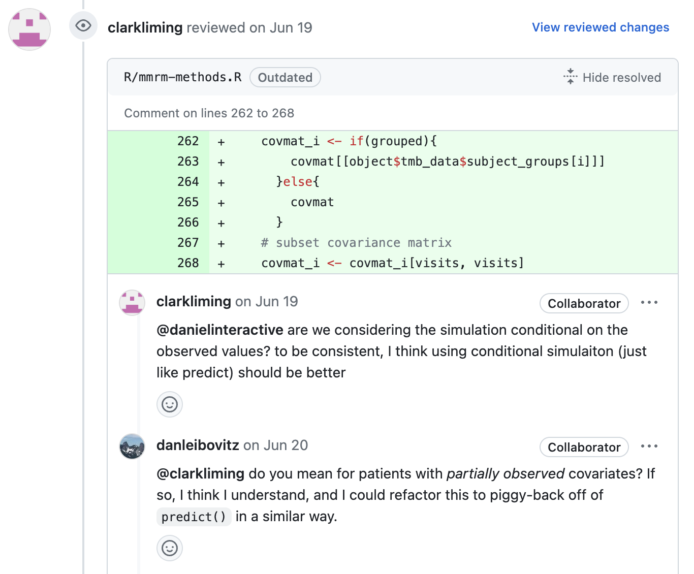
5. Merge 🎉
When all concerns have been addressed, new code is introduced.

Workflow Recap
- Discussion preceeds work on new features
- Alignment is emphasized at Bi-weekly calls before embarking on development
- Volunteer-based implmentation, depending on availability, expertise and interest
- Calls allow for intermitent feedback throughout - especially important for larger features
- PR submitted, with appropiately intensive review
- When concerns are addressed, feature is incorporated
What we covered today
- Show practical steps for obtaining an R package implementation of a statistical method
- Discuss key considerations for writing statistical software
- Illustrate throughout with the
mmrmpackage development example
- Short hands-on introduction to the
mmrmpackage- Working together across companies and in open source
Special Thanks to All of {mmrm}’s Contributors
- Daniel Sabanes Bove (Roche)
- Julia Dedic (Roche)
- Doug Kelkhoff (Roche)
- Kevin Kunzmann (Boehringer Ingelheim)
- Brian Matthew Lang (Merck)
- Liming Li (Roche)
- Christian Stock (Boehringer Ingelheim)
- Ya Wang (Gilead)
- Craig Gower-Page (Roche)
- Dan James (Astrazeneca)
- Jonathan Sidi (pinpointstrategies)
- Daniel Leibovitz (Roche)
- Daniel D. Sjoberg (Roche)
From the statistical method to the R package - the mmrm example | License